How to visualise the results in OVITO
The SKMF software's output file is in extended .XYZ file format that contains every recorded state of the simulated system. To visualize the results we recommend OVITO, The Open Visualization Tool which is available to all major operating systems, including Microsoft Windows, MacOS and Linux.
A. Stukowski, Visualization and analysis of atomistic simulation data with OVITO - the Open Visualization Tool, Modelling Simul. Mater. Sci. Eng. 18 (2010), 015012
Download OVITO
Download the current stable version (2.6.2 on 28/04/2016) of OVITO from the following link:
http://ovito.org/index.php/download
Extract the downloaded compressed file and run the executable ovito file.
Load File
The first step when using OVITO is to load the simulation data to be visualized. OVITO can read several file formats and will try to detect the format of a file automatically.
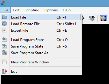
To load the simulation results into OVITO select the File → Load File command from the main menu, or the corresponding button in the toolbar (or Ctrl+I).
Column mapping
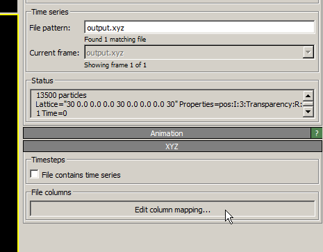
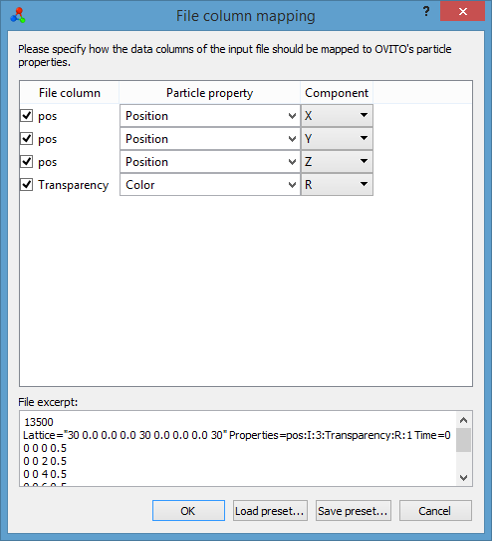
After opening the data file, a file column mapping dialog pops up, letting you assign data columns stored in the file to particle properties. The default SKMF software assigns the columns automatically as x,y,z coordinates and transparency which represents the composition. The dialog can be accessed also by pressing the Edit column mapping... button on the right side of the main window at the bottom.
The first three columns are the coordinates of the atoms, for these select Position.
The fourth column corresponds to the composition at each site. Select either Color, Transparency or Radius for different types of visualizations. Click OK.
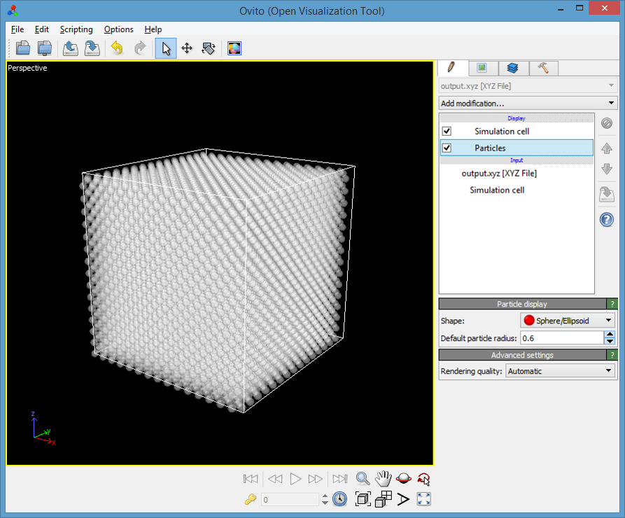
After File column mapping you are now back to OVITO's main window.
Navigation and display
The viewports display three-dimensional views of the simulation snapshot that you just loaded. Every viewport can be moved independently. You can rotate the image by left clicking on it and moving the mouse while keeping the button down. With the same action but with right clicking you can move the image up-down and left-right. One also can zoom in the viewport under the cursor by turning the wheel of the mouse. To maximize one of the viewports, click on it, then press the ![]() button in the bottom row. You can also find dedicated buttons there for the above-mentioned actions, rotation, translation and zoom.
button in the bottom row. You can also find dedicated buttons there for the above-mentioned actions, rotation, translation and zoom.
One can change the radius of the spheres representing the atoms by clicking on the Particles row on the right side of the window and changing the value of Default particle radius.
Loading time series
Up until now OVITO showed only the initial state of the system we simulated. To load all the recorded states of the system stored in the file, one must click on the output.xyz [XYZ file] line on the right side of the window, and tick the box of File contains time series option right above the Edit column mapping... button.

After this step one can use the slider under the viewports to choose a recorded state to show or press the triangle-shaped play button to watch the whole process as an animation.
Color coding
For better visualization one can use the Color coding modifier. On the right hand side of the window click on the drop-down menu of Add modification... and choose Color coding. It assigns a color to each atom based on the value of another property of that atom. In the sub-menu Property: select the property you assigned to the fourth, composition column at the column mapping step.

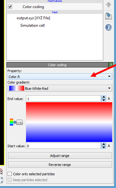
It's important to note that Color coding doesn't affect the selected property (except color, obviously), so this way one can represent the composition at the sites as e.g. the radius and the color of the spheres at the same time, which options used wisely can result in 3D figures that are easier to take in and understand.
One can change the color gradients from a drop-down menu or even load custom color maps. The values that the two ends of the color scale represents can be changed, too. Every value that are over or under of the given range will be represented by the upper or lower end of the color map, accordingly.

Slicing the sample
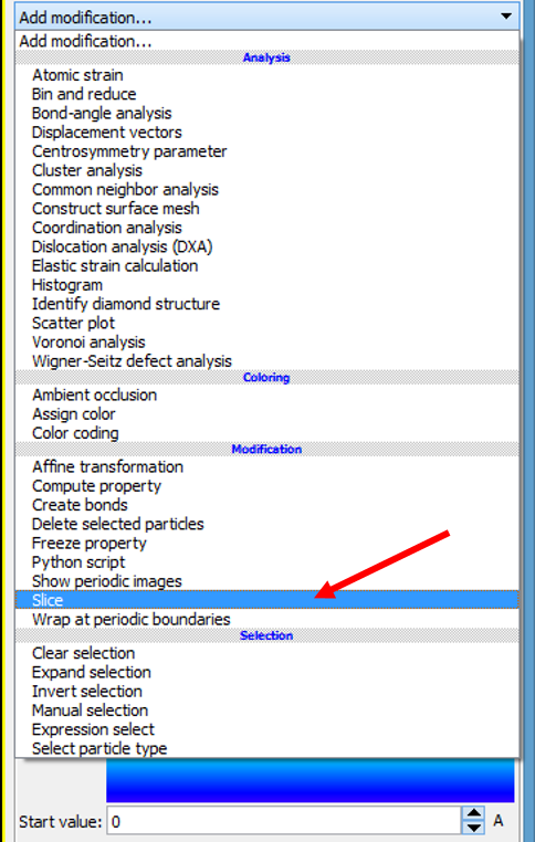
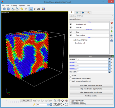
From the several modifier options of OVITO we'd like to mention one more. The Slice modifier cuts away all atoms on one side of an infinite plane in space, or shows only the particles within a slice of certain width. It can be used to create cross sections or slices of the sample.
More options
OVITO has many more visual and also analytical options. Detailed explanations can be found on the project's site: http://ovito.org/index.php/about/features .